Terms used in Cell Entries in Table 9-1

Interpolation

Interpolation is literally involved in figuring out an intermediate value. Neighboring values are mobilized to determine the value desired. Usually a value is required for a given point (as in deteriming a grid of values from a scattered collection of points), but interpolation can also be used to determine the position of a given value (as in locating a contour). Rules like MAXIMUM value wouldn't make much sense as an "intermediate" value; Interpolation is usually about retaining the smoothness and pretending that you have measurements at locations where you don't. (This CAN be valid, if your assumptions about the behavior of surfaces make sense...)

Interpolation: Unit 40 from NCGIA core curriculum; the Illinois (was Corps of Engineers) visualization group (web-site not responding); one of their papers;

Kinds of Interpolation

• Linear: assumes a proportional distance relationship between a particular pair of points; generalizes to triangles (assumed to be flat). RETAINS all data values.
• IDW (Inverse Distance Weighting): (see an old Exercise 6)
  • Assembles a "neighborhood" of a few points, can use a fixed radius, or a target number of points (expanding and contracting to reflect density).
  • Computes new value from those in neighborhood, weighted so that farthest points contribute least. May decline as 1/distance, 1/distance squared, etc. (This is the POWER parameter)
  • Will retain values at all points (since distance goes to zero, and inverse distance goes infinite...) BUT distance within a cell is non-zero... [example of interpolation differences]
• SYMAP [dead computer mapping program Version 5 written in 1968, had marvelous interpolation by D. Shepherd] (variant of IDW, min and max # of points) actually added "intervening opportunity" (decreased weights if a point was closer in a given sector...). BARRIERS: spatial limits on assembling points
• Splines: use a numerical model based on an idealized thin spring.
  • As programmed in GRASS, has a tension parameter and a smoothing parameter. If smoothing set to zero, retains values. [NOTE: these web links dead, sadly]
  • Spline in ArcMap has "weight value" (taughtness), number of points, select either "regularized" or "tension"... (see Geospatial Analyst extension)
• Trend surfaces: fit a polynomial of some degree (linear, parabolic, cubic, etc.) to all the points. STRONG assumption that the overall trend is more important than the particular values.
• Kriging (optimal interpolation); based on covariance as well as value; uses decline of correlation with distance (semivariance)... [an animated GIF; a full textbook chapter ; examples: eco-risk assessment (benthic species), indicator kriging for Chernobyl (ArcGeostatistical Analyst); precipitation in Slovenia; all big .pdfs]

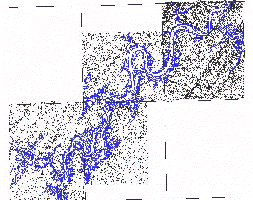
Examples of Interpolation

• From isoline to DEM By way of sampling points along the contours then to DEM
• From scattered points to DEM; Result for river segments
• the GRASS visualization group (web-site not responding); one of their papers
• comparison of various interpolation methods (listed above);
• a paper about fiddling with the parameters of interpolation
• Trend surface capabilities of IDRISI
• example of trend surface (Kansas)

Tracing

Tracing involves constructing a smooth contour that passes through the points that have been interpolated. Tracing can be as simple as linear segments across triangles, or use a spline to pass a curve or a given 'tension' through all the points with proper continuity.

Examples of Tracing

• Constructing isolines through DEM (visualization) [dead]

Version of 14 November 2002