Objectives of lecture:
The Dane County Project has examples of complex transformations
between physical model of soil erosion and planning perspectives
of ownership. (mentioned in Lecture 1, revisited - a few slides)
Textbook includes three examples:
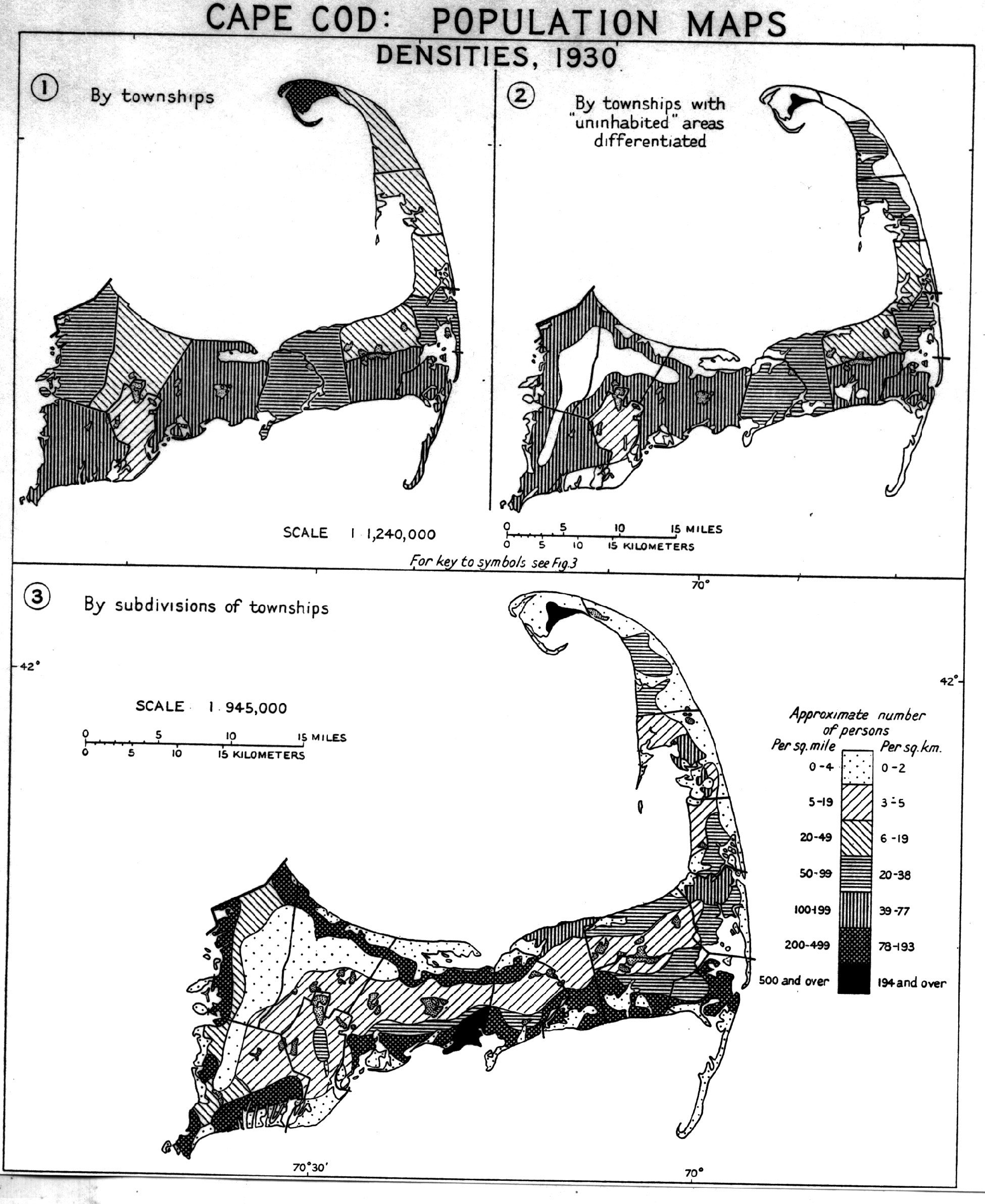
John K. Wright 1936 Cape Cod
Wright wanted to produce a map of population density that reflected
the places people actually lived. He only had population by TOWN.
So, he constructed a land use map, and tried to generate a reasonable
density to assign to each land use class. He then took the total
town population and allocated it to the various land use zones
in the town.
This method he termed dasymetric meaning that it mapped
density.
Cartographers continue to cite Wright's 1936 study, and ascribe
a kind of 'integrated survey' logic to the boundaries that appear.
They misunderstand Wright's use of two map sources. The land use
map was used because Wright assumed that the same class had similar
densities in adjacent towns, thus permitting him to estimate the
density from the sources he had. His study was a form of areal interpolation, but also a case
of some tricky use of sparse data to solve a set of simultaneous
linear equations...
Wisconsin statutes set up two regimes to recognize wetlands.
The first works through the assessment of parcels, while
the second works through an inventory of wetlands.
To examine the effectiveness of these two programs to serve as
reciprocal 'carrot and stick', the two views of the landscape
must be combined. A transformation of wetland acreage onto the
parcels demonstrates that there are some large discrepencies between
the two processes. (more SLIDES)
Information from two radically different resolution remote sensing systems are used to estimate the percentage of forest cover. A selected set of more detailed TM images (30 m pixels) are used to calibrate the relationship between forests and the 1 km pixels of AHVRR. The regression analysis is performed separately on each of the 15 "physiographic regions" of Hammond's regionalization of the 48 states. The result of percent forest cover per 1 km pixel, based on the spectral values of that pixel and the regression analysis for the physiographic region. [Overheads]
See Zhu and Evans, 1994: US Forest types and Predicted percent
forest cover from AVHRR data, Photogrammetric Engineering and
Remote Sensing, 60(5), 525-531.
Or the .pdf
version of the Southern Forest Experiment Station report SO-280.
The combination of geometric (neighborhood) processing and attribute combinations can be applied to the operations studied in earlier chapters and lectures.
What appears to be "data" is actually the result of some prior operation(s) (transformation(s)).
For example: bat diversity on Cape York, Queensland. Bat observations were POINTS (one dead bat, each classified as to species) then a new geometry was imposed (30 minute grid). The attribute rule was count of distinct species (TOTAL rule).
Roughly speaking two groups of spatial processing procedures: Local (containers) and Neighborhoods
Actually a form of spatial JOIN where the "key" is sharing position (containership)
Simple form of container: Point in Polygon
More complicated: Polygon Overlay
Actual all served by one engine that performs "Planar Enforcement" on the geometry
Reaching out from the local, various techniques
Forms of Aggregation
Forms of Disaggregation
Assumption of uniformity depends on measurement scale (an example of how derived ratios are really different from "raw" values like counts.) and it depends on what spatial units are considered.